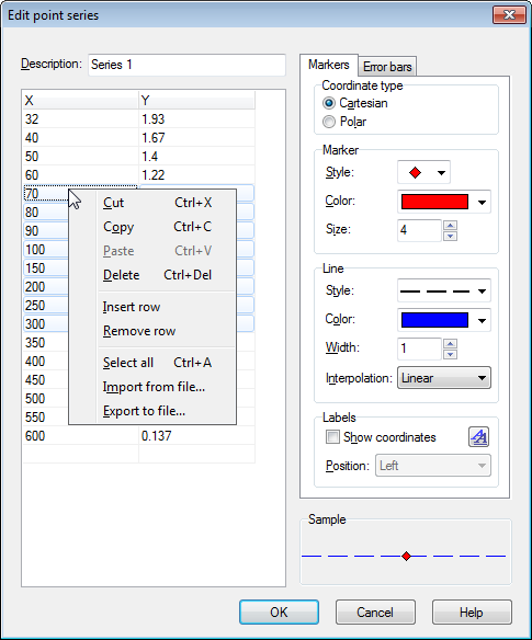
You can use the dialog below to add a series of points to the coordinate system. The points will be shown in the coordinate system in the graphing area as a series of markers. To insert a new point series, you use → . To change an existing point series, you first select it in the function list and use → .
After adding a point series, you may add a trendline which is the curve of best fit for the points.
In the grid you can enter the x- and y-coordinates of the points. You may enter any number of points you want, but all points need both an x-coordinate and a y-coordinate.
You can select some points and use the right click menu to copy them to another program. Likewise you may copy data from other programs like MS Word or MS Excel and paste them into this the grid in dialog.
From the context menu, you can also choose to import data from a file. Graph can import text files with data separated by either tabs, commas or semicolons. The data will be placed at the position of the caret. This makes it possible to load data from more than one file, or to have x-coordinates in one file and y-coordinates in another file. In the usual case where you have all data in one file, you should make sure that the caret is located at the upper left cell before you import.
- Description
In the edit box at the top of the dialog, you can enter a name for the series, which will be shown in the legend.
- Coordinate type
You need to choose between the type of coordinates used for the points. Cartesian is used when you want to specify (x,y)-coordinates. Polar is used when you want to specify (θ,r)-coordinates, where θ is the angle and r is the distance from the origin. The angle θ is in radians or degrees depending on the current setting.
- Marker
To the right you can choose between different types of markers. The style may be a circle, a square, a triangle, etc. You may also change the color and size of the markers. If the size is set to 0, neither markers nor error bars will be shown.
Notice that if you select an arrow as marker, the arrow will be shown pointing tangential to the line at the point. The actual direction therefore depends on the Interpolation setting. The first point is never shown when the marker is an arrow.
- Line
It is possible to draw lines between the markers. The line will always be drawn between points in the same order they appear in the grid. You can choose between different styles, colors and widths for the lines. You can also choose to draw no line at all.
You can choose between four types of interpolation: Linear will draw straight lines between the markers. 1D cubic spline will draw a natural cubic spline, which is a nice smooth line connecting all the points sorted by the x-coordinate with 3rd degree polynomials. 2D cubic spline will draw a smooth cubic spline through all points in order. Half cosine will draw half cosine curves between the points, which might not look as smooth as the cubic splines but they never undershoot/overshoot like the cubic splines can do.
- Labels
Put a check in Show coordinates to show Cartesian or polar coordinates at each point. You may use the
 button to change the font, and the drop down box to select whether the labels are shown over, below, to the left or to the right of the points.
- Error bars
Here you can choose to show horizontal or vertical error bars, also known as uncertainty bars. They are shown as thin bars at each point in the point series indicating the uncertainty of the point. There are three ways to indicate the size of the error bars: Fixed is used to specify that all points have the same uncertainty. Relative is used to specify a percentage of the x- or y-coordinate for each point as uncertainty. Custom will add an extra column to the table where you may specify a different uncertainty value for each point. All uncertainties are ±values. Custom Y-errors are also used to weight the points when creating trendlines.